2nd Place Solution: LLM Decoders, Assignment Optimization, and Custom Post-Processing

Originally published as a Kaggle writeup for the h2o.ai Predict the LLM competition.

In this post I would like to present our team’s solution write-up that finished 2nd place (public 2nd place) in the “h2o.ai Predict the LLM” competition on Kaggle. We would like to express our thanks to the Kaggle team, to h2o.ai, and to all fellow competitors for such a short-lived joyful experience during the 2 weeks of this state-of-the-art hackathon.

Personally, I also would like to thank my teammate Kha for our short but fruitful collaboration. Hope we can work together in another competition soon.

In short, here are the 2 major ideas that mainly contributed to our success:

1. Finetune an LLM decoder with a classification head with the competition’s data.
2. Optimize the prediction (binarizing it using linear assignment optimization method), then combine this binary prediction with the original raw prediction with custom post-processing steps.

1. The LLM Models (Binga)

On Kaggle, it’s established that encoders, such as DeBERTa, have ruled NLP competitions on Kaggle for years. To brush up my NLP skills, I joined this competition on day 1 and started with encoders. I realized that simple DeBERTa models scored in the range of 1.6, 1.4 on mlogloss metric.

1.1 Model Selection

Given that it’s 2023 and we have new decoders coming out almost each day, I decided to use a decoder model out of sheer curiosity. Now, which models do we begin with? I went with the most popular Mistral model for 2 reasons: 1) Performance. It outperforms Llama2-13b on some benchmarks, and 2) Apache 2.0 License.

1.2 Experiments

Each of the experiments were done on H2O-LLMStudio. It’s a fantastic no-code tool to quickly run experiments with many LLMs. Highly recommend having this tool in your data science toolbox.

Coming to experiments, with Mistral-Instruct-v0.1, my local validation loss dramatically reduced and the leaderboard score fell from 1.6 to 1.063. This seemed like the right direction as psi’s benchmark was 0.88 and we’re getting there. A little bit of tuning with epochs and I got 0.925 on LB. I tried modifying int4/int8/bfloat16 finetuning, LoRA parameters and always saw an adverse effect. One of the key parameters that improved my score was prompt length, answer length. The more they are, the better the logloss. This was easy to explain as some of the sentences (specifically answers) were longer than 2000 in length.

One of the interesting parameters is the seed. Fixing the seed led to deterministic results but a random seed resulted in a different logloss and LB score. The variance is 0.05 which is extremely high in this competition. This led to the conclusion that averaging multiple models was the way to go to fight variance.

Along the way, I clustered the data to visually explore it using cluestar library and found that GroupKFold was the way to go. This was a moment of personal learning that “explore the data first before modeling”.

1.3 Open Models

With huggingface hosting so many models, the open_llm_leaderboard shows top models based on benchmark scores. Motivated to further improve the score, I tried multiple models finetuned on top of Mistral and while some worked, some did not.

1.4 Averaging

Lastly, these models were not perfectly correlated and that led to nice performance on averaging. So, a straight average of predictions (not oof predictions) from the 9 models below, with different seeds, led to 0.63 on the leaderboard.

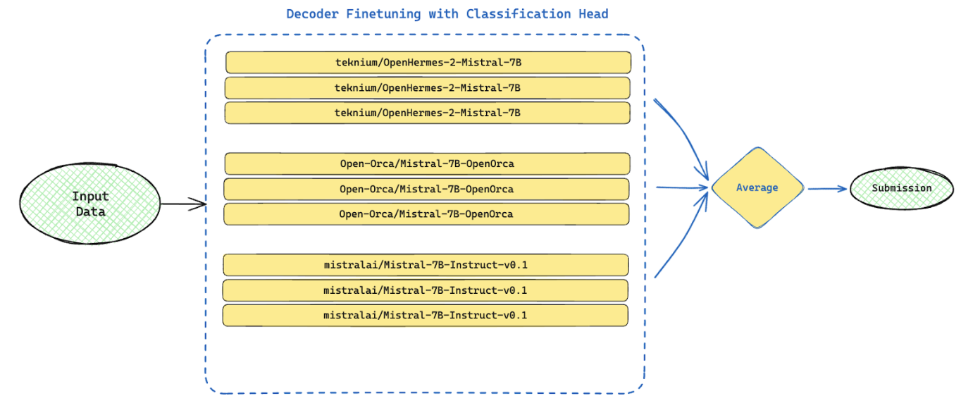Decoder Finetuning with Classification Head – 9 models averaged for final submission

5 days prior to the competition end, Kha and I decided to team up and his optimization work (details in the next section) was a big part of this solution going from 0.63 to 0.50 on the public leaderboard.

1.5 Infrastructure

All the decoder models were trained on a machine with 8 x V100 GPUs. This meant that each finetuning run approximately took around 60 minutes along with inference on test data.

1.6 Note from binga

A big thanks to H2O.ai, Kaggle and the organizers for setting up this wonderful competition where I learnt so much about SoTA NLP.

Thanks to AI practitioners in open source who are behind projects such as Open Hermes, Open Orca etc for making these great models available to us.

Special thanks to Kha for giving me an opportunity to team up with him! I’ve learnt so much from Kha – understanding data, doing quick experiments and most importantly a never-say-die attitude in the last 2 days when we were challenged by competitors such as Reacher and that made us push ourselves during the last hours.

2. Optimization and Post-Processing (Kha)

This competition’s data has a very special trait, that for each question group, we should expect exactly 1 response for each of 7 label targets. During the normal modeling process, we may not exploit any of this extra information about relation between data samples.

This sparks an idea of using an optimization method to find the best assignment of targets for a group of 7 responses to a specific question. The optimization method takes as input a 7x7 matrix, where each row is the normalized probability (sum to 1) of 1 data sample. We then try to maximize the selected probabilities given the constraint that each target must be assigned exactly one time.

This optimization method alone, however, cannot outperform the original predictions due to its extreme nature (of hard 0/1 prediction) that can’t drive the log-loss down. So I need to perform some more extra steps of combining this binary prediction (also a 7x7 matrix) with the original matrix. The combining steps and optimization coefficients were achieved manually by a systematic search to minimize the out-of-fold predictions. The single steps of post-processing are shown in the function below.

You may wonder why there are some highly manual steps. In general, they are just the results of the following ideas:

• The highest prediction within 1 data sample (a row) should come to 1
• All the other 6 predictions within that data sample should come to 0
• The above 2 ideas can only be implemented after the assignment optimization step.

The optimization function is highly customized and straightforward, that can be applied to any submission!

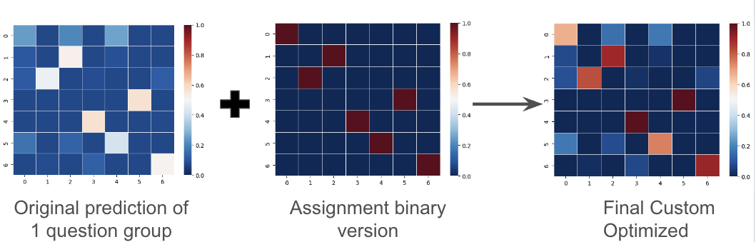Original prediction + Assignment binary version = Final Custom Optimized

def optim(df1, pred):
    for q, _df in df1.groupby('Question'):

        # Stage 1 optim
        indices = _df.index.values
        cost_matrix = -pred[indices]
        row_idx, col_idx = linear_sum_assignment(cost_matrix)
        orig = pred[indices]
        hard_pred = np.zeros((7,7))
        hard_pred[row_idx, col_idx] = 1
        hard_pred_minus = 1-hard_pred

        orig_selected = np.zeros((7,7))
        orig_selected[row_idx, col_idx] = orig[row_idx, col_idx]
        orig_unselected = orig.copy()
        orig_unselected[row_idx, col_idx] = 0
        soft_pred_1 = orig_selected + (hard_pred-orig_selected)*0.005
        soft_pred_2 = orig_unselected - orig_unselected**1.475
        soft_pred = soft_pred_1 + soft_pred_2
        pred[indices] = soft_pred

        # Stage 2 optim
        for jcol in range(7):
            max_idx = np.argmax(soft_pred[:, jcol])
            if max(soft_pred[:, jcol]) > 1:
                soft_pred[:, jcol] = 0.01
                soft_pred[max_idx, jcol] = 0.99
            elif max(soft_pred[:, jcol]) > 0.67:
                soft_pred[:, jcol] -= soft_pred[:, jcol]*0.715
                soft_pred[max_idx, jcol] += (1-soft_pred[max_idx, jcol])*0
            elif max(soft_pred[:, jcol]) > 0.245:
                soft_pred[:, jcol] -= soft_pred[:, jcol]*0.56
                soft_pred[max_idx, jcol] += (1-soft_pred[max_idx, jcol])*0

        pred[indices] = soft_pred

    return pred

optimized_preds = optim(test, probabilities)

3. Other Ideas That Also Worked (Kha)

Sidelining the main 2 major factors presented, I also experimented with some other classical approaches and found out that they worked nicely, but I couldn’t find the time to combine that with Phani’s because Phani cannot produce the out-of-fold predictions on time. My methods highly depend on the train out-of-fold predictions. Even the binary classification idea and post-process was based on my out-of-fold deberta-v3-large predictions, instead of the best Phani’s LLM model. Had the optimization been tuned on the latter, we would have a better final score I’m pretty sure.

3.1 LightGBM Stacking

Using a tree-based method (LightGBM) to learn a stacking model on top of the NLP predictions. The crafted features that helped are:

• Gpt_rating: asking another LLM to rate the response within a fixed scale.
• Statistics (mean, median, min, max, std) of some main features (text length, gpt_rating) aggregated by each question’s group
• Category of each question: asking another LLM to categorize each question into a few categories such as: biology, history, math, idea, recommendation…

This modeling process boosted my raw deberta-v3-large score of 1.1 to about 0.950.

3.2 Pseudo-labeling

Using the test prediction as the additional training data isn’t a new idea. But in this competition it won’t give any benefits given the log-loss metric (binarize the prediction hurts the score, hence additional data is indeed detrimental).

However if the binarized version is retrieved (simply by using an argmax function) after being optimized and post-processed (as described in section 2), pseudo-label will work. However (again), the training process with pseudo-labels is not straightforward, because if we train on full test data in any session, the knowledge cannot improve and the test prediction itself finally is biased to its original version, giving no benefit.

So I have to train a k-fold on the question (suppose k=5), do the split on the train data, and also do the split on the pseudo data. In a single fold training, the 4/5 parts of train data plus the 4/5 parts of pseudo data will serve as training data, the 1/5 remaining part of train data will serve as validation data, and the 1/5 remaining part of pseudo data will serve as test data (that needs prediction). This strategy can ensure that the test prediction on the 1/5 test part will not have bias towards its existing target knowledge.

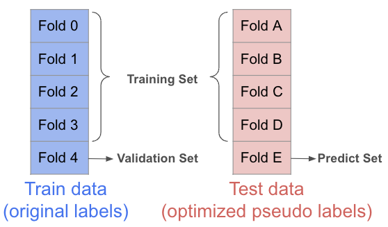K-fold pseudo-labeling: train data with original labels + test data with optimized pseudo labels

With pseudo training and LightGBM modeling, I observed a nice-size score boost of about 0.1 to 0.15 on the raw deberta-v3-large submission. But as Phani didn’t generate out-of-fold LLM predictions so I couldn’t implement these two methods although I have the code.

3.3 Conclusive Remarks

We may have a significantly better score that could break 0.499 if we combine all of the ideas together, like in these steps:

1. Step 1: Train a decoder LLM, predict the out-of-fold along with test predictions.
2. Step 2: Train a LightGBM model on top of step 1, with the hand-crafted features.
3. Step 3: Optimize and post-process the predictions from step 2.
4. Step 4: Use the test predictions from step 3 as the additional training data, repeat from step 1.

Our full code is at: https://www.kaggle.com/khahuras/2nd-place-solution